11Алгоритмы планирования процессов fcfs, Round Robin, sjf, их сравнение, преимущества, недостатки.
Недостатки: Процесс, ограниченный возможностями процессора может затормозить более быстрые процессы, ограниченные устройствами ввода/вывода.
Прямой порядок выполнения (оказался неэффективным — процессы долго находятся в состоянии готовности).
Прямой порядок выполнения (более эффективный чем первый).
Циклическое планирование RR (Round Robin)
Самый простой алгоритм планирования и часто используемый.
Каждому процессу предоставляется квант времени процессора. Когда квант заканчивается процесс переводится планировщиком в конец очереди. При блокировке процессор выпадает из очереди.
Преимущества: Простота Справедливость (как в очереди покупателей, каждому только по килограмму)
Недостатки: Если частые переключения (квант — 4мс, а время переключения равно 1мс), то происходит уменьшение производительности.
Если редкие переключения (квант — 100мс, а время переключения равно 1мс), то происходит увеличение времени ответа на запрос.
Модификацией алгоритма FCFS является алгоритм, получивший название Round Robin (Round Robin – это вид детской карусели в США) или сокращенно RR. По сути дела, это тот же самый алгоритм, только реализованный в режиме вытесняющего планирования. Можно представить себе все множество готовых процессов организованным циклически – процессы сидят на карусели. Карусель вращается так, что каждый процесс находится около процессора небольшой фиксированный квант времени, обычно 10 – 100 миллисекунд. Пока процесс находится рядом с процессором, он получает процессор в свое распоряжение и может исполняться.
На производительность алгоритма RR сильно влияет величина кванта времени. Рассмотрим тот же самый пример с порядком процессов p0, p1, p2 для величины кванта времени, равной 1. Время ожидания для процессаp составит 5 единиц времени, для процесса p1 – тоже 5 единиц, для процесса p2 – 2 единицы. В этом случае среднее время ожидания получается равным (5 + 5 + 2)/3 = 4 единицам времени. Среднее полное время исполнения составит (18 + 9 + 3)/3 = 10 единиц времени.
Shortest-Job-First (SJF)
Кратчайшая задача — первая
Преимущества: Уменьшение оборотного времени
Справедливость (как в очереди покупателей, кто без сдачи проходит в перед)
Недостатки: Длинный процесс занявший процессор, не пустит более новые краткие процессы, которые пришли позже (в случае невытесняющего).
SJF-алгоритм краткосрочного планирования может быть как вытесняющим, так иневытесняющим. При невытесняющем SJF-планировании процессор предоставляется избранному процессу на все необходимое ему время, независимо от событий, происходящих в вычислительной системе. При вытесняющем SJF-планировании учитывается появление новых процессов в очереди готовых к исполнению (из числа вновь родившихся или разблокированных) во время работы выбранного процесса.
Scheduling Algorithms in Operating System
In the operating system, everything is carried out by processes. At any given time, there is only one process that is running on the CPU. A process scheduler removes one process from the running state in the CPU and selects another process to run based on some scheduling algorithms in OS.
What is a Scheduling Algorithm?
A CPU scheduling algorithm is used to determine which process will use CPU for execution and which processes to hold or remove from execution. The main goal or objective of CPU scheduling algorithms in OS is to make sure that the CPU is never in an idle state, meaning that the OS has at least one of the processes ready for execution among the available processes in the ready queue.
There are two types of scheduling algorithms in OS:
Preemptive Scheduling Algorithms
In these algorithms, processes are assigned with priority. Whenever a high-priority process comes in, the lower-priority process that has occupied the CPU is preempted. That is, it releases the CPU, and the high-priority process takes the CPU for its execution.
Non-Preemptive Scheduling Algorithms
In these algorithms, we cannot preempt the process. That is, once a process is running on the CPU, it will release it either by context switching or terminating. Often, these are the types of algorithms that can be used because of the limitations of the hardware.
There are some important terminologies to know for understanding the scheduling algorithms:
Arrival Time: This is the time at which a process arrives in the ready queue.
Completion Time: This is the time at which a process completes its execution.
Burst Time: This is the time required by a process for CPU execution.
Turn-Around Time: This is the difference in time between completion time and arrival time. This can be calculated as:
Turn Around Time = Completion Time – Arrival Time
Waiting Time: This is the difference in time between turnaround time and burst time. This can be calculated as:
Waiting Time = Turn Around Time – Burst Time
Throughput: It is the number of processes that are completing their execution per unit of time.
Why Do We Need Scheduling?
A process to complete its execution needs both CPU time and I/O time. In a multiprogramming system, there can be one process using the CPU while another is waiting for I/O whereas, in a uni programming system, time spent waiting for I/O is completely wasted as the CPU is idle at this time. Multiprogramming can be achieved by the use of process scheduling.
The purposes of a scheduling algorithm are as follows:
- Maximize the CPU utilization, meaning that keep the CPU as busy as possible.
- Fair allocation of CPU time to every process
- Maximize the Throughput
- Minimize the turnaround time
- Minimize the waiting time
- Minimize the response time
Types of Scheduling Algorithms in OS
First Come First Serve (FCFS) Scheduling Algorithm
First Come First Serve is the easiest and simplest CPU scheduling algorithm to implement. In this type of scheduling algorithm, the CPU is first allocated to the process which requests the CPU first. That means the process with minimal arrival time will be executed first by the CPU. It is a non-preemptive scheduling algorithm as the priority of processes does not matter, and they are executed in the manner they arrive in front of the CPU. This scheduling algorithm is implemented with a FIFO(First In First Out) queue. As the process is ready to be executed, its Process Control Block (PCB) is linked with the tail of this FIFO queue. Now when the CPU becomes free, it is assigned to the process at the beginning of the queue.
Advantages
- Involves no complex logic and just picks processes from the ready queue one by one.
- Easy to implement and understand.
- Every process will eventually get a chance to run so no starvation occurs.
Disadvantages
- Waiting time for processes with less execution time is often very long.
- It favors CPU-bound processes then I/O processes.
- Leads to convoy effect.
- Causes lower device and CPU utilization.
- Poor performance as the average wait time is high.
Shortest Job First (SJF) Scheduling Algorithm
Shortest Job First is a non-preemptive scheduling algorithm in which the process with the shortest burst or completion time is executed first by the CPU. That means the lesser the execution time, the sooner the process will get the CPU. In this scheduling algorithm, the arrival time of the processes must be the same, and the processor must be aware of the burst time of all the processes in advance. If two processes have the same burst time, then First Come First Serve (FCFS) scheduling is used to break the tie.
The preemptive mode of SJF scheduling is known as the Shortest Remaining Time First scheduling algorithm.
Advantages
- Results in increased Throughput by executing shorter jobs first, which mostly have a shorter turnaround time.
- Gives the minimum average waiting time for a given set of processes.
- Best approach to minimize waiting time for other processes awaiting execution.
- Useful for batch-type processing where CPU time is known in advance and waiting for jobs to complete is not critical.
Disadvantages
- May lead to starvation as if shorter processes keep on coming, then longer processes will never get a chance to run.
- Time taken by a process must be known to the CPU beforehand, which is not always possible.
RoundRobin Scheduling Algorithm
The Round Robin algorithm is related to the First Come First Serve (FCFS) technique but implemented using a preemptive policy. In this scheduling algorithm, processes are executed cyclically, and each process is allocated a small amount of time called time slice or time quantum. The ready queue of the processes is implemented using the circular queue technique in which the CPU is allocated to each process for the given time quantum and then added back to the ready queue to wait for its next turn. If the process completes its execution within the given quantum of time, then it will be preempted, and other processes will execute for the given period of time. But if the process is not completely executed within the given time quantum, then it will again be added to the ready queue and will wait for its turn to complete its execution.
The round-robin scheduling is the oldest and simplest scheduling algorithm that derives its name from the round-robin principle. In this principle, each person will take an equal share of something in turn.
This algorithm is mostly used for multitasking in time-sharing systems and operating systems having multiple clients so that they can make efficient use of resources.
Advantages
- All processes are given the same priority; hence all processes get an equal share of the CPU.
- Since it is cyclic in nature, no process is left behind, and starvation doesn't exist.
Disadvantages
- The performance of Throughput depends on the length of the time quantum. Setting it too short increases the overhead and lowers the CPU efficiency, but if we set it too long, it gives a poor response to short processes and tends to exhibit the same behavior as FCFS.
- The average waiting time of the Round Robin algorithm is often long.
- Context switching is done a lot more times and adds to the overhead time.
Shortest Remaining Time First (SRTF) Scheduling Algorithm
Shortest Remaining Time First (SRTF) scheduling algorithm is basically a preemptive mode of the Shortest Job First (SJF) algorithm in which jobs are scheduled according to the shortest remaining time. In this scheduling technique, the process with the shortest burst time is executed first by the CPU, but the arrival time of all processes need not be the same. If another process with the shortest burst time arrives, then the current process will be preempted, and a newer ready job will be executed first.
Advantages
- Processes are executed faster than SJF, being the preemptive version of it.
Disadvantages
- Context switching is done a lot more times and adds to the overhead time.
- Like SJF, it may still lead to starvation and requires the knowledge of process time beforehand.
- Impossible to implement in interactive systems where the required CPU time is unknown.
Master the complexities of operating systems with Scaler Topics Free certification course. Join now & learn the foundations of the operating system.
Process Scheduling Algorithms-FCFS,SJF,Priority & Round Robin
A Process Scheduler schedules different processes to be assigned to the CPU based on particular scheduling algorithms. There are six popular process scheduling algorithms which we are going to discuss in this chapter −
- First-Come, First-Served (FCFS) Scheduling
- Shortest-Job-Next (SJN) Scheduling
- Priority Scheduling
- Shortest Remaining Time
- Round Robin(RR) Scheduling
- Multiple-Level Queues Scheduling
These algorithms are either non-preemptive or preemptive. Non-preemptive algorithms are designed so that once a process enters the running state, it cannot be preempted until it completes its allotted time, whereas the preemptive scheduling is based on priority where a scheduler may preempt a low priority running process anytime when a high priority process enters into a ready state.
First Come First Serve (FCFS)
- Jobs are executed on first come, first serve basis.
- It is a non-preemptive, pre-emptive scheduling algorithm.
- Easy to understand and implement.
- Its implementation is based on FIFO queue.
- Poor in performance as average wait time is high.
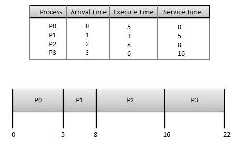
Wait time of each process is as follows −
| Process | Wait Time : Service Time – Arrival Time |
|---|---|
| P0 | 0 – 0 = 0 |
| P1 | 5 – 1 = 4 |
| P2 | 8 – 2 = 6 |
| P3 | 16 – 3 = 13 |
Average Wait Time: (0+4+6+13) / 4 = 5.75
Shortest Job Next (SJN)
- This is also known as shortest job first, or SJF
- This is a non-preemptive, pre-emptive scheduling algorithm.
- Best approach to minimize waiting time.
- Easy to implement in Batch systems where required CPU time is known in advance.
- Impossible to implement in interactive systems where required CPU time is not known.
- The processer should know in advance how much time process will take.
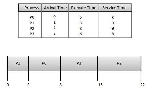
Wait time of each process is as follows −
| Process | Wait Time : Service Time – Arrival Time |
|---|---|
| P0 | 3 – 0 = 3 |
| P1 | 0 – 0 = 0 |
| P2 | 16 – 2 = 14 |
| P3 | 8 – 3 = 5 |
Average Wait Time: (3+0+14+5) / 4 = 5.50
Priority Based Scheduling
- Priority scheduling is a non-preemptive algorithm and one of the most common scheduling algorithms in batch systems.
- Each process is assigned a priority. Process with highest priority is to be executed first and so on.
- Processes with same priority are executed on first come first served basis.
- Priority can be decided based on memory requirements, time requirements or any other resource requirement.
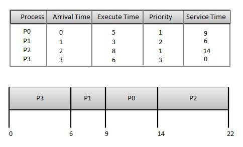
Wait time of each process is as follows −
| Process | Wait Time : Service Time – Arrival Time |
|---|---|
| P0 | 9 – 0 = 9 |
| P1 | 6 – 1 = 5 |
| P2 | 14 – 2 = 12 |
| P3 | 0 – 0 = 0 |
Average Wait Time: (9+5+12+0) / 4 = 6.5
Shortest Remaining Time
- Shortest remaining time (SRT) is the preemptive version of the SJN algorithm.
- The processor is allocated to the job closest to completion but it can be preempted by a newer ready job with shorter time to completion.
- Impossible to implement in interactive systems where required CPU time is not known.
- It is often used in batch environments where short jobs need to give preference.
Round Robin Scheduling
- Round Robin is the preemptive process scheduling algorithm.
- Each process is provided a fix time to execute, it is called a quantum.
- Once a process is executed for a given time period, it is preempted and other process executes for a given time period.
- Context switching is used to save states of preempted processes.
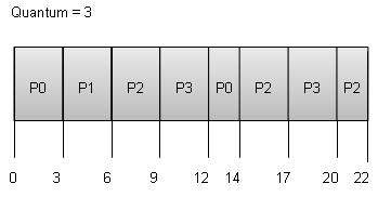
Wait time of each process is as follows −
| Process | Wait Time : Service Time – Arrival Time |
|---|---|
| P0 | (0 – 0) + (12 – 3) = 9 |
| P1 | (3 – 1) = 2 |
| P2 | (6 – 2) + (14 – 9) + (20 – 17) = 12 |
| P3 | (9 – 3) + (17 – 12) = 11 |
Average Wait Time: (9+2+12+11) / 4 = 8.5
Multiple-Level Queues Scheduling
Multiple-level queues are not an independent scheduling algorithm. They make use of other existing algorithms to group and schedule jobs with common characteristics.
- Multiple queues are maintained for processes with common characteristics.
- Each queue can have its own scheduling algorithms.
- Priorities are assigned to each queue.
For example, CPU-bound jobs can be scheduled in one queue and all I/O-bound jobs in another queue. The Process Scheduler then alternately selects jobs from each queue and assigns them to the CPU based on the algorithm assigned to the queue.
Fcfs round что это
In a system, there are a number of processes that are present in different states at a particular time. Some processes may be in the waiting state, others may be in the running state and so on. Have you ever thought how CPU selects one process out of some many processes for execution? Yes, you got it right. CPU uses some kind of process scheduling algorithms to select one process for its execution amongst so many processes. The process scheduling algorithms are used to maximize CPU utilization by increasing throughput. In this blog, we will learn about various process scheduling algorithms used by CPU to schedule a process.
But before starting this blog, if you are not familiar with Burst time, Arrival time, Exit time, Response time, Waiting time, Turnaround time, and Throughput, then you should first learn these topics by reading the blog from here . Also, learn about Preemptive and Non-Preemptive scheduling from here .
Since you are done with the prerequisites of this blog, let’s get started by learning different process scheduling algorithms.
First Come First Serve (FCFS)
As the name suggests, the process coming first in the ready state will be executed first by the CPU irrespective of the burst time or the priority. This is implemented by using the First In First Out (FIFO) queue. So, what happens is that, when a process enters into the ready state, then the PCB of that process will be linked to the tail of the queue and the CPU starts executing the processes by taking the process from the head of the queue (learn more about PCB from here ). If the CPU is allocated to a process then it can’t be taken back until it finishes the execution of that process.

In the above example, you can see that we have three processes P1, P2, and P3, and they are coming in the ready state at 0ms, 2ms, and 2ms respectively. So, based on the arrival time, the process P1 will be executed for the first 18ms. After that, the process P2 will be executed for 7ms and finally, the process P3 will be executed for 10ms. One thing to be noted here is that if the arrival time of the processes is the same, then the CPU can select any process.
Advantages of FCFS:
- It is the most simple scheduling algorithm and is easy to implement.
Disadvantages of FCFS:
- This algorithm is non-preemptive so you have to execute the process fully and after that other processes will be allowed to execute.
- Throughput is not efficient.
- FCFS suffers from the Convey effect i.e. if a process is having very high burst time and it is coming first, then it will be executed first irrespective of the fact that a process having very less time is there in the ready state.
Shortest Job First (Non-preemptive)
In the FCFS, we saw if a process is having a very high burst time and it comes first then the other process with a very low burst time have to wait for its turn. So, to remove this problem, we come with a new approach i.e. Shortest Job First or SJF.
In this technique, the process having the minimum burst time at a particular instant of time will be executed first. It is a non-preemptive approach i.e. if the process starts its execution then it will be fully executed and then some other process will come.

In the above example, at 0ms, we have only one process i.e. process P2, so the process P2 will be executed for 4ms. Now, after 4ms, there are two new processes i.e. process P1 and process P3. The burst time of P1 is 5ms and that of P3 is 2ms. So, amongst these two, the process P3 will be executed first because its burst time is less than P1. P3 will be executed for 2ms. Now, after 6ms, we have two processes with us i.e. P1 and P4 (because we are at 6ms and P4 comes at 5ms). Amongst these two, the process P4 is having a less burst time as compared to P1. So, P4 will be executed for 4ms and after that P1 will be executed for 5ms. So, the waiting time and turnaround time of these processes will be:
Advantages of SJF (non-preemptive):
- Short processes will be executed first.
Disadvantages of SJF (non-preemptive):
- It may lead to starvation if only short burst time processes are coming in the ready state(learn more about starvation from here ).
Shortest Job First (Preemptive)
This is the preemptive approach of the Shortest Job First algorithm. Here, at every instant of time, the CPU will check for some shortest job. For example, at time 0ms, we have P1 as the shortest process. So, P1 will execute for 1ms and then the CPU will check if some other process is shorter than P1 or not. If there is no such process, then P1 will keep on executing for the next 1ms and if there is some process shorter than P1 then that process will be executed. This will continue until the process gets executed.

In the above example, at time 1ms, there are two processes i.e. P1 and P2. Process P1 is having burst time as 6ms and the process P2 is having 8ms. So, P1 will be executed first. Since it is a preemptive approach, so we have to check at every time quantum. At 2ms, we have three processes i.e. P1(5ms remaining), P2(8ms), and P3(7ms). Out of these three, P1 is having the least burst time, so it will continue its execution. After 3ms, we have four processes i.e P1(4ms remaining), P2(8ms), P3(7ms), and P4(3ms). Out of these four, P4 is having the least burst time, so it will be executed. The process P4 keeps on executing for the next three ms because it is having the shortest burst time. After 6ms, we have 3 processes i.e. P1(4ms remaining), P2(8ms), and P3(7ms). So, P1 will be selected and executed. This process of time comparison will continue until we have all the processes executed. So, waiting and turnaround time of the processes will be:
Advantages of SJF (preemptive):
- Short processes will be executed first.
Disadvantages of SJF (preemptive):
- It may result in starvation if short processes keep on coming.
Round-Robin
In this approach of CPU scheduling, we have a fixed time quantum and the CPU will be allocated to a process for that amount of time only at a time. For example, if we are having three process P1, P2, and P3, and our time quantum is 2ms, then P1 will be given 2ms for its execution, then P2 will be given 2ms, then P3 will be given 2ms. After one cycle, again P1 will be given 2ms, then P2 will be given 2ms and so on until the processes complete its execution.
It is generally used in the time-sharing environments and there will be no starvation in case of the round-robin.

In the above example, every process will be given 2ms in one turn because we have taken the time quantum to be 2ms. So process P1 will be executed for 2ms, then process P2 will be executed for 2ms, then P3 will be executed for 2 ms. Again process P1 will be executed for 2ms, then P2, and so on. The waiting time and turnaround time of the processes will be:
Advantages of round-robin:
- No starvation will be there in round-robin because every process will get chance for its execution.
- Used in time-sharing systems.
Disadvantages of round-robin:
- We have to perform a lot of context switching here, which will keep the CPU idle(learn more about context switching from here ).
Priority Scheduling (Non-preemptive)
In this approach, we have a priority number associated with each process and based on that priority number the CPU selects one process from a list of processes. The priority number can be anything. It is just used to identify which process is having a higher priority and which process is having a lower priority. For example, you can denote 0 as the highest priority process and 100 as the lowest priority process. Also, the reverse can be true i.e. you can denote 100 as the highest priority and 0 as the lowest priority.

In the above example, at 0ms, we have only one process P1. So P1 will execute for 5ms because we are using non-preemption technique here. After 5ms, there are three processes in the ready state i.e. process P2, process P3, and process P4. Out to these three processes, the process P4 is having the highest priority so it will be executed for 6ms and after that, process P2 will be executed for 3ms followed by the process P1. The waiting and turnaround time of processes will be:
Advantages of priority scheduling (non-preemptive):
- Higher priority processes like system processes are executed first.
Disadvantages of priority scheduling (non-preemptive):
- It can lead to starvation if only higher priority process comes into the ready state.
- If the priorities of more two processes are the same, then we have to use some other scheduling algorithm.
Multilevel Queue Scheduling
In multilevel queue scheduling, we divide the whole processes into some batches or queues and then each queue is given some priority number. For example, if there are four processes P1, P2, P3, and P4, then we can put process P1 and P4 in queue1 and process P2 and P3 in queue2. Now, we can assign some priority to each queue. So, we can take the queue1 as having the highest priority and queue2 as the lowest priority. So, all the processes of the queue1 will be executed first followed by queue2. Inside the queue1, we can apply some other scheduling algorithm for the execution of processes of queue1. Similar is with the case of queue2.
So, multiple queues for processes are maintained that are having common characteristics and each queue has its own priority and there is some scheduling algorithm used in each of the queues.

In the above example, we have two queues i.e. queue1 and queue2. Queue1 is having higher priority and queue1 is using the FCFS approach and queue2 is using the round-robin approach(time quantum = 2ms).
Since the priority of queue1 is higher, so queue1 will be executed first. In the queue1, we have two processes i.e. P1 and P4 and we are using FCFS. So, P1 will be executed followed by P4. Now, the job of the queue1 is finished. After this, the execution of the processes of queue2 will be started by using the round-robin approach.
Multilevel Feedback Queue Scheduling
Multilevel feedback queue scheduling is similar to multilevel queue scheduling but here the processes can change their queue also. For example, if a process is in queue1 initially then after partial execution of the process, it can go into some other queue.
In a multilevel feedback queue, we have a list of queues having some priority and the higher priority queue is always executed first. Let’s assume that we have two queues i.e. queue1 and queue2 and we are using round-robin for these i.e. time quantum for queue1 is 2 ms and for queue2 is 3ms. Now, if a process starts executing in the queue1 then if it gets fully executed in 2ms then it is ok, its priority will not be changed. But if the execution of the process will not be completed in the time quantum of queue1, then the priority of that process will be reduced and it will be placed in the lower priority queue i.e. queue2 and this process will continue.
While executing a lower priority queue, if a process comes into the higher priority queue, then the execution of that lower priority queue will be stopped and the execution of the higher priority queue will be started. This can lead to starvation because if the process keeps on going into the higher priority queue then the lower priority queue keeps on waiting for its turn.
This is all about process scheduling algorithms. That’s it for this blog. Hope you learned something new today.
Do share this blog with your friends to spread the knowledge. Visit our YouTube channel for more content. You can read more blogs from here .